It's a Bird, It's a Plane!

The Data

• Stanford STL-10 dataset
• 10 classes: airplane, bird, car, cat, deer, dog, horse, monkey, ship, truck
• 96x96 px, 3 channel RGB images
• 500 training images, 800 test images per class
• 100000 unlabeled images for unsupervised learning

The Process

Grayscale

Color is not generally a useful feature for object classification. This is because objects often have a more consistent shape than color, and it is likely that the training data will not contain a full sampling of colors. So, the first step is to convert all images to grayscale.

Features

Next, images often contain too much unnecessary visual complexity, so feeding the raw pixels into classifying models rarely produces ideal results, especially in the types of models I’m working with on this project. (Things might be different if I were using certain types of neural networks)

Harris Corners

Pros:

• Easy to understand (they’re corners, as in where two edges meet)
• Somewhat customizable (you can set a threshold to determine roughly how many corners you detect in a given image)

Cons:

• Sensitive to noise/patterns (notice the chain link fence behind the cat in the fourth image)

I ultimately decided against using these for my final models

SIFT (Scale-Invariant Feature Transform)

• Proprietary (David Lowe, 1999/2004)
• More confusing than corners (Difference of Gaussians to generate feature vectors in 128 dimensional space)
• Work well. Sift features are often good at handling identification of objects even when they are partially obscured or viewed from strange angles.

SIFT features are what I decided to work with for this project, though I also just wanted to gain experience working with them, since they are known to work well and are used in industry.

Since there can be a somewhat arbitrary number of features per image, it is necessary to do further processing in order to get to data that can be fed to a model. I clustered the features with k-means clustering over a variety of ks (number of clusters) and training images, since I wasn’t sure of the ideal number of clusters. I then computed feature occurrence histograms by calculating the frequency with which specific features were assigned to given clusters. These histograms were then fed to a series of models for training and testing. Ideally, I would have used k nearest neighbors as a model as well, but it was taking too long to train and test.

The Results (confusion matrix)

This confusion matrix shows my classification results across different models, numbers of training images, and feature clusters. The rows are the actual image labels, the columns are the predicted labels, each cell shows the percent of images of that row label that were classified as a given column label. This means that the true positives (correct classifications) are along the diagonal and everything else is a misclassification.

Image classification is hard

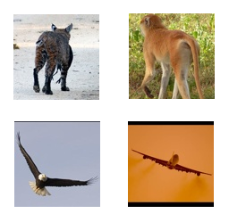
The most difficult class in general seems to be birds, and they are often classified as airplanes. It’s not too hard to think why this might be, but the confusion matrix for the Gaussian Naive Bayes model shows that sometimes cats and monkeys are classified as each other. This might seem more strange, until you look at some of the training images.
Cat-Monkey and Bird-Plane:

Some images are just odd. A couple of these made me take a second look at their assigned labels. Can you classify them? (results on hover)

Results and Other Research

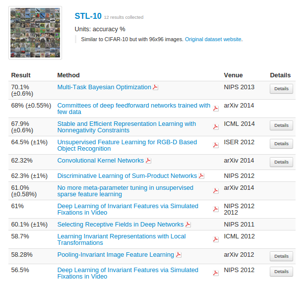
My best models are over three times better than guessing, and, according to this website, I happened to pick a fairly difficult dataset. I also didn’t get time to address the unlabeled images, which is where this dataset really excels. I guess I’ll just have to experiment with deep learning next time!